A friend had a back log of hand made habitat maps that needed digitising into vector and raster maps for further analysis. They asked me how this might be done. After a bit of searching and playing around on QGIS I came up with a protocol and decided to put together a tutorial.
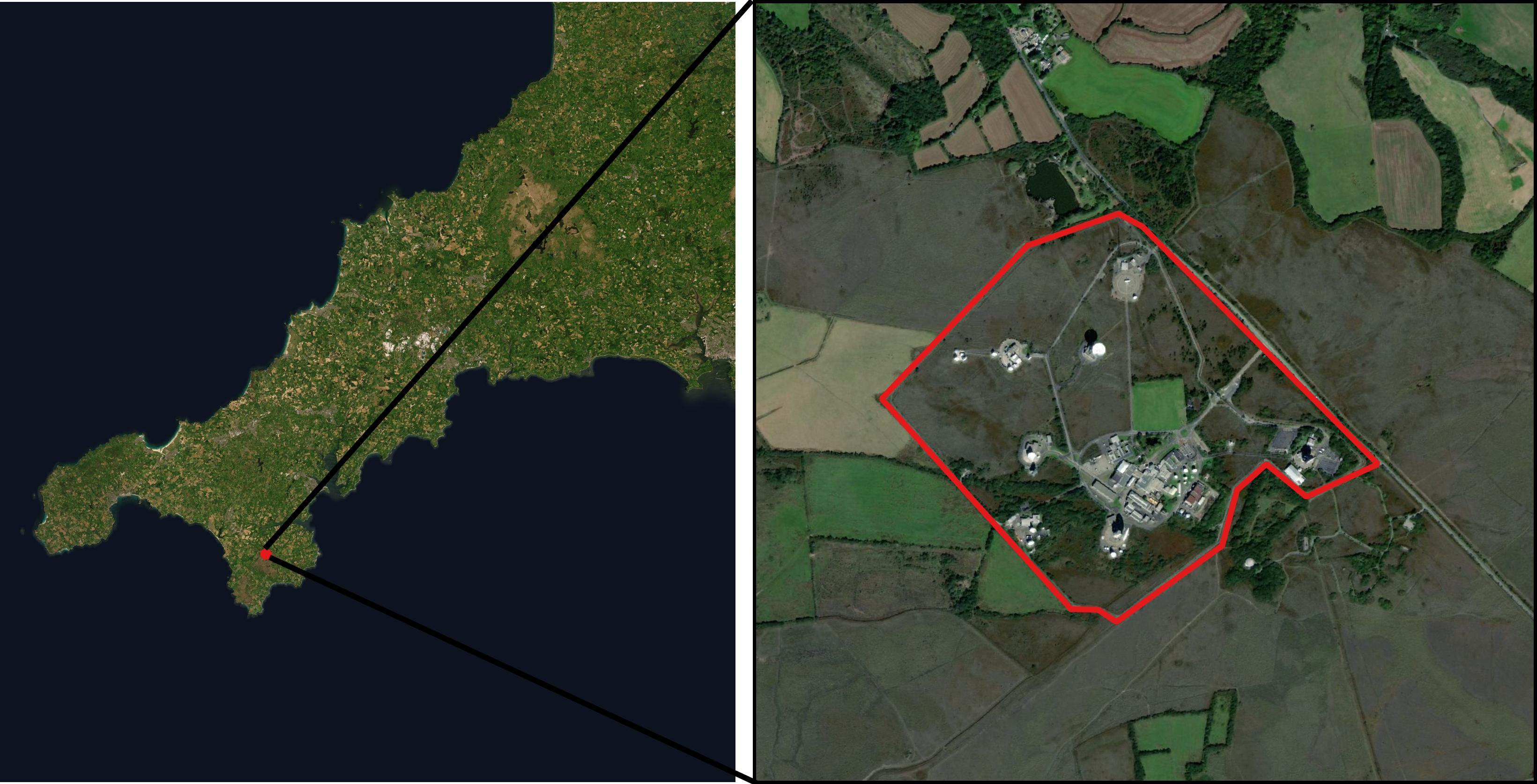
The tutorial involves some fictitious data I made for Goon Hilly in Cornwall. After making a .shp file of the area of interest, I gridded it off, printed it out and coloured in the grid with three colours to make a habitat map. I then made a second habitat map with a fourth colour to represent the urban infrastructure. The maps were then scanned in and can be downloaded (below) in the tutorial.
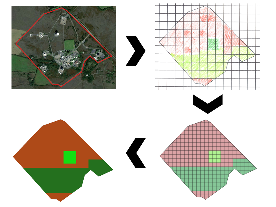
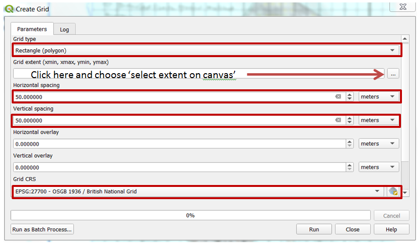
1. import the files 2. Georeference the PDF of the scanned habitat maps 3. Create a grid 4. Vectorise the habitat types 5. Create a raster

i. right click the layer, select properties then symbology ii. Click 'colour' iii. Change the opacity to something between 0-40%
a. Click Raster > Georeferencer (if this is not an option head to Plugins > manage and install plugins, search for Georeferencer, select/install it and the option should now be visible) b. Open the scanned image 'Habitat_map1.PDF'; File > open raster c. Click the 'add point' tool and select a point on the image to reference. Try to select an obvious part of the polygon boundary such as an edge with a strong angle. d. After selecting a point to reference a window will pop up. Select the ‘From map canvas’ button and then click on the corresponding edge of the .shp file and then click 'OK'.
i. Transformation type = Linear ii. Resampling method = Nearest neighbour iii. Target SRS = Project CRS iv. Output raster; click the dotted button to assign the file path and nameg. Click the 'Start georeferencing' button to finish. h. Compare the boundaries to make sure the scanned image has been geo-referenced adequately enough. If not, repeat the process with more points.
i. Open the Grid layers attribute table (right click layer and select ‘open attribute table). ii. Click the 'toggle editing' button iii. Click the 'new field' button and add a text field called ‘Habitat’ with a length of ~20 characters iv. Add another field that is an integer called ‘HabitatID’ with a length of ~3 characters.d. Select the grid squares to assign a habitat type e.g. gorse or heather:
i. Go back to the main window and click the 'select features by area or single click' button, then select the grid squares you want to assign to a particular habitat by either dragging the mouse over them or holding ctrl and clicking on multiple grid squares.e. Assign the habitat type:
i. Click Edit > modify attributes of selected features ii. Enter the habitat and habitatID to the relevant fields. NOTE: Keep a record of the numbers you assign habitats so the coding system can be replicated in subsequent maps.f. Fill all grid squares and then toggle out of editing mode to save the layer
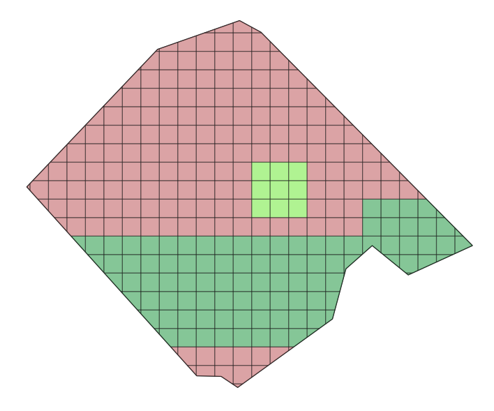
i. Right click the layer and go to properties, then symbology. Change ‘single symbol’ to ‘categorized’, change the column to the ‘Habitat’ column and then click classify. ii. Change the empty field (by right clicking it) to 100% opacity so only the grid outlines can be seen.
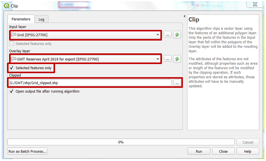
i. Input = clipped grid layer ii. Field = Habitat ID (numeric field) iii. Output raster size units = Georeferenced units iv. resolution = 1 (otherwise the grid squares may shift a few pixels) v. Output extent = click the dotted button and select ‘use layer extent’ and choose the clipped grid layer v vi. In the advanced parameters section, enter the file name and locationc. Colour raster:
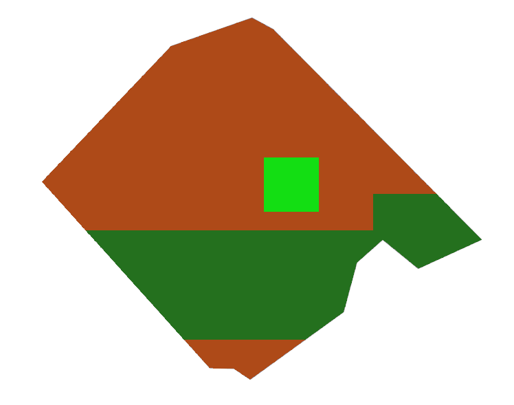
i. Right click raster layer, then properties, then symbology ii. Change render type to Paletted/unique values and click classify. iii. You can then right click the categories to change the colours to a desired palette which can be saved for later use.Now do it all again for the second habitat map. Remember, you can import the georeferenced points that were saved in step 2. If the points do not line up on the scanned image you can click the 'move point' button to move the points to the correct places.